Ibis is a mature open-source project that has been in development for about 5 years; it currently has about 1350 stars on Github. It provides an interface to SQL for Python programmers and bridges the gap between remote storage & execution systems. These features provide authors the ability to:

1. write backend-independent SQL expressions in Python;
2. access different database connections (eg. SQLite, OmniSci, Pandas); and
3. confirm visually their SQL queries with directed acyclic graphs (DAGs).

Ibis is an alternative approach using databases that relies on Python rather than SQL experience. Typically, users have to learn an entirely new syntax or flavor of SQL to perform simple tasks. Now, those familiar with Python can avoid a new learning curve by using Ibis for composing and executing database queries using familiar Python syntaxes (i.e., similar to Pandas and Dask). Ibis assists in formation of SQL expressions by providing visual feedback about each Python object. This post focuses on writing SQL expressions in Python and how to compose queries visually using Ibis. We'll demonstrate this with a SQLite database---in particular, Sean Lahman's baseball database.

Connecting to a database

To get started, we'll need to establish a database connection. Ibis makes it easy to create connections of different types. Let's go ahead and do this now with the function ibis.sqlite.connect (in this instance, the database used is a SQLite database):

The client object represents our connection to the database. It is essential to use the appropriate Ibis connection---SQLite in this case constructed through the ibis.sqlite namespace---for the particular database.

This baseball database has 29 distinct tables; we can see by running the following code:

This database has 29 tables.

Selecting and visualizing tables

Displaying the list tables, gives the names of all the tables which include, among others, tables with identifiers

Let's use the database connection to extract & examine dataframe representations of the halloffame and appearances tables from the baseball database. To do this, we can invoke the table method associated with the client object called with the appropriate names.

At the moment, the objects objects halloffame and appearances just constructed don't hold any data; instead, the objects are expressions of type TableExpr that represent putative operations applied to the data. The data itself is inert wherever it's actually located---in this case, within the SQLite database. We can verify this by examining their types or by using assertions like this:

The object appearances has type TableExpr.

We can examine the contents of these Ibis table expressions using the TableExpr.limit or the TableExpr.head method (similar to the Pandas DataFrame.head method). That is, we can define an object sample that represents a sub-table comprising the first few rows of the halloffame table:

The object sample is of type TableExpr

Remember, the object sample is a TableExpr object representing some SQL query to extracts a sub-table from a larger table. We can view the actual SQL query corresponding to sample by compiling it with the compile method and converting the result to a string:

'SELECT t0."ID", t0."playerID", t0.yearid, t0."votedBy", t0.ballots, t0.needed, t0.votes, t0.inducted, t0.category, t0.needed_note \nFROM base.halloffame AS t0\n LIMIT ? OFFSET ?'

Another useful feature of Ibis is its ability to represent an SQL query as a DAG (Directed Acyclic Graph). For instance, evaluating the object sample at the interactive command prompt yields a visualization of a sequence of database operations:

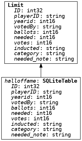
This image of a DAG is produced using Graphviz; those familiar with Dask may have used a similar helpful feature to assemble task graphs.

Finally, the actual sub-table corresponding to the expression sample can be extracted using the execute method (similar to compute in Dask). The result returned by executing the expression sample is a tidy Pandas DataFrame object.

The type of result is DataFrame

A similar extraction of the leading five rows from the appearances table (in one line) gives the following table with 23 columns:

Filtering and selecting data

As mentioned earlier, Ibis uses familiar Pandas syntax to build SQL queries. As an example, let's look at the various kinds of entries in the category column from the halloffame table. A nice way to do this is to extract the relevant column with attribute access and apply the value_counts method. Remember, an invokation of execute is needed to realize the actual expression.

There are four different types of entries in this column, most of which are Players. To illustrate filtering and selection, we'll create a expression condition of boolean values corresponding to rows from the halloffame table in which the category column has the value Player. The boolean values represented by condition can be extracted from the table halloffame using brackets. The final result is bound to the identifier players.

Joining Ibis tables

If we want a single view of the halloffame players and their appearances, we need to join the tables halloffame and appearances. To do this, we'll perform an inner join based on the playerID columns of our players & appearances tables.

We notice that both the players and the appearances tables each have a column labelled ID. This column needs to be excluded from appearances; otherwise the overlapping columns will corrupt the computed join. Specifically, we want to filter out the ID and playerID columns from the appearances table. One strategy to do this is to use a list comprehension.

Now, we use the TableExpr.join method to compute an inner join of the players table and the filtered appearances table; the result is bound to the identifier unmaterialized.

Materializing the join

We used the identifier unmaterialized just above to emphasize that the resulting expression is not a materialized view (that would be required to build new expressions). Without a materialized view, Ibis raises an exception (as demonstrated here).

Unable to execute "unmaterialized.distinct()" IbisError('Table operation is not yet materialized')

The distinct method in the preceding code behaves like the Pandas DataFrame.drop_duplicates method, i.e., it drops duplicated rows. We can obtain such a materialized view to circumvent the exception above using the expression's materialize method.

The code above completes the join and binds the resulting expression to the materialized object join; here is a sample of the leading five rows of our joined data (notice the result has 31 columns).

Ibis supports other join strategies as methods of the class TableExpr. The following list comprehension shows us what they are.

['anti_join', 'any_inner_join', 'any_left_join', 'asof_join', 'cross_join', 'inner_join', 'join', 'left_join', 'outer_join', 'semi_join']

Executing an expression

We'll now expand the expression join as a Pandas DataFrame object. We'll use this DataFrame to answer the following question:

Some of the "hitters" have also been "pitchers", so we'll need to filter out rows corresponding to those appearances from the table join. That is, to identify a specific player as a "pitcher", we'll choose those players who played mostly as pitchers; in particular, we'll take 100 games as an arbitrary threshold between pitchers and non-pitchers. The column G_p from the table join represents the numbers of games a player played as a pitcher; the desired filtering expression, then, is as follows:

Next, we group the pitchers table based on a specific pair of columns (stored as a list cols) and then count them annually using a groupby with a count aggregation.

The expression grouped_pitchers is still an Ibis TableExpr; as we've seen several times now, it can be realized as a Pandas DataFrame using the execute method. The resulting DataFrame's index can be set as a multi-index using the inducted and yearID columns.

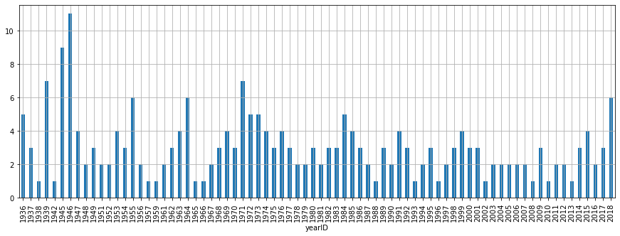
The dataframe df has counts of the number of pitchers who were (inducted index 'Y') and were not (inducted index 'N') inducted into the baseball Hall of Fame in a given year. We'll pull in all the relevant counts of inductees into a dataframe count_inducted_pitchers. Notice the use of the Pandas DataFrame.fillna method to assign 0s in rows appropriately (i.e., reflecting that no pitchers were inducted into the Hall of Fame in those years).

The Pandas DataFrame & Series classes have a convenient plotting interface. We'll use a dictionary options to specify keyword arguments to tidy the final invokation of plot.bar.

What next?

That's it! In future posts, we'll explore other backends and visualize more Ibis objects. If you'd like to contribute to Ibis, please take a look at Ibis contributing guide and OpenTeams.